
Fatigue is the Initiation, formation and propagation of cracks in a material due to cyclic loads. These cyclic loads lead to repeated stresses and if material is subjected to such repeated stresses, the components fail at stresses below the yield point stresses. Such type of failure of material is Fatigue failure. The fatigue of material is affected by various factors such as the number of load reversals, irregularities, size of the component, relative magnitude of fluctuating loads, etc. There are few important concepts used in fatigue analysis are discussed below:
Endurance Limit or Fatigue Limit
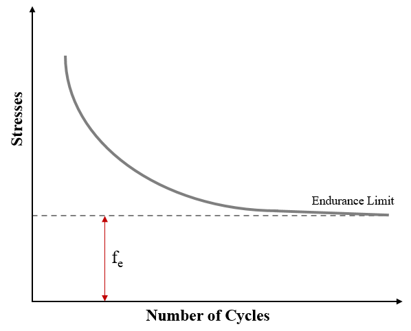
The Figure 1 shows the Stress Vs Number of cycle graphs. In this graph, if the stress is kept below a certain value (dotted line) the material (component) will not fail. This stress as represented by the dotted line is known as a fatigue limit (fe) or endurance limit. The Fatigue limit or Endurance limit is the stress level below which an infinite number of loading cycles can be applied to a material without causing fatigue failure. When a material is subjected to a stress that is lower than its endurance limit, it should theoretically be able to withstand an indefinite amount of load cycles.
Fatigue Loading Types
The time based loading have mainly two types as discussed below:
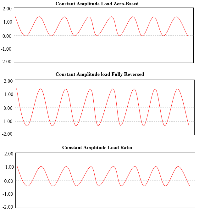
1. Constant Amplitude loading:
Here, the maximum and minimum stress levels are constant. This is the simplest case and has different loading type options; Such as Zero-based, Fully Reversed and Ratio (R-ratio). Refer Figure 2 for constant loading type options.
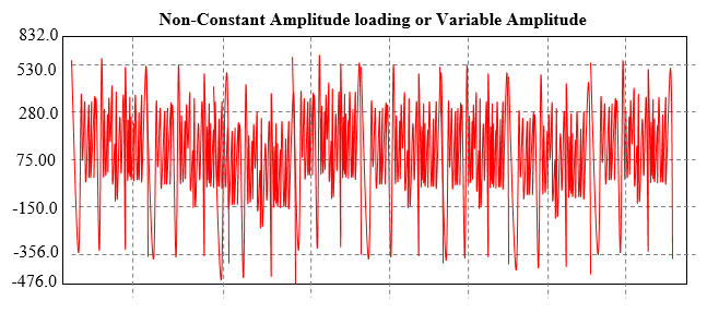
2. Variable Amplitude or Non-constant loading:
In this case, as name suggest the loads are not constant but varying drastically.
Furthermore, Loadings are classified as proportional and non-proportional loading;
Proportional loading: It means, the ratio of principal stresses is constant and principal stress does not change over time.
Non-proportional loading: It means that there is no relationship between the stress components. The typical examples are nonlinear boundary conditions, alternating between two different load cases, alternating load superimposed on a static load, etc.
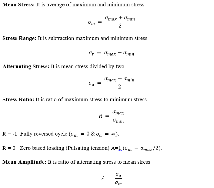
Important Definitions:
This paragraphs discussed various terminology used in fatigue analysis.
Mean Stress Theories:
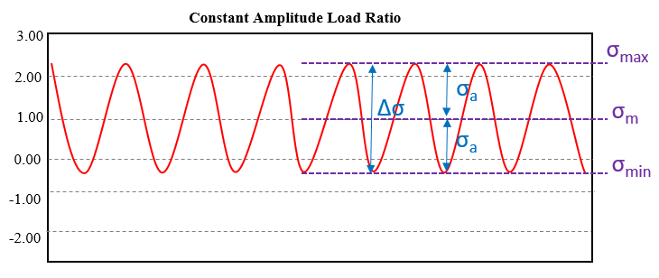
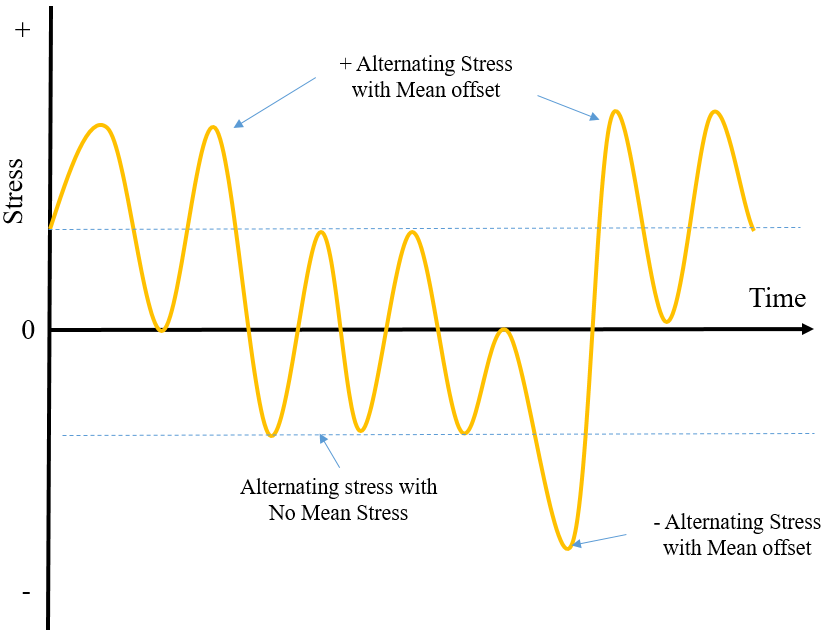
Fatigue failure happens when a component is subjected to repeated cyclic loads. These cyclic loads forms stress cycle’s resulting alternating stresses which causes the fatigue damage. Nevertheless, the amount of damage caused does not only depend on alternating stress but also mean stress.
In real world, the loads coming on product used are not constant but varying as shown in Figure 5. Some cycles have mean offset or some does not have; accordingly alternating stress may also vary.
The SN curves are obtained by applying the cyclic loading to a laboratory specimen. The typical loading is either pure axial or bending and reflects uniaxial state of stress. For multiple cycle, multiple tests are required to get SN curves which are under different mean stress conditions; which takes times and efforts. So, instead of shifting SN-Curve to account for mean stresses, a more common procedure is to transform the rainflow matrix of the load time history, which contains all the stress cycle information for a given load time history.
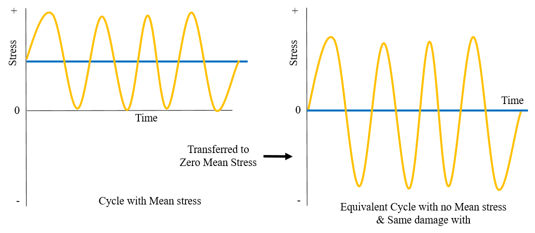
Mean Stress Correction:
A mean stress correction is used to transform a stress cycle to an equivalent stress cycle with zero mean stress as sown in Figure 6. The transformed stress cycle must still contain the same fatigue damage potential.
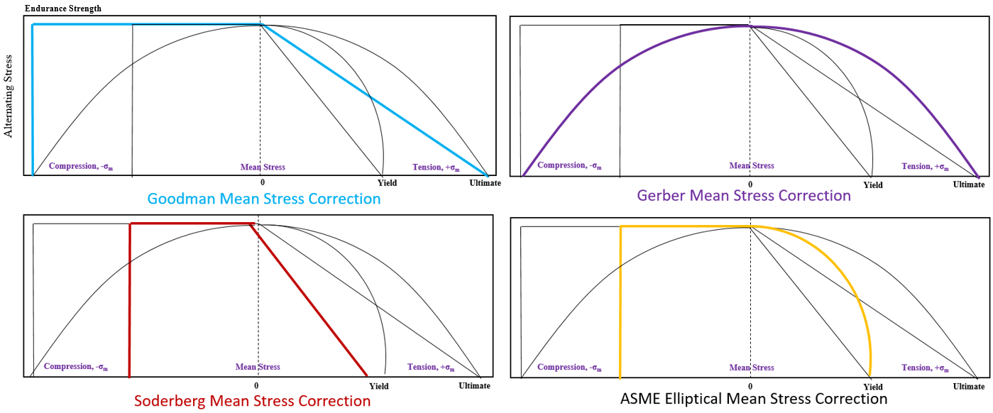
Mean Stress Correction Methods:
Goodman, Soderberg, Ferber and ASME Elliptical are different mean stress correction theories. Figure 7 shows all mean stress correction theories; in this graph, the right hand side shows compressive mean stress while left hand are tensile mean stresses.
- Goodman Method: A straight line connecting the endurance limit and the ultimate strength (on positive) follows the suggestion of Goodman. A Goodman line is used when the design is based on ultimate strength and may be used for ductile or brittle materials. Refer blue colour line for Goodman mean stress correction. In this, no correction is done on compressive mean stresses.
- Soderberg Method: Soderberg criteria is defined as the straight line joining on stress amplitude axis and on mean stress axis. Refer red colour line from below graph, it is more conservative than Goodman theory and sometime used for brittle materials.
- Gerber Method: Gerber parabola refers to the parabolic line joining two points in x axis (σut) and y axis (σw). According to the Gerber criteria, the region below this curve is considered to be safe. It provides a good fit for ductile metals for tensile mean stresses while incorrectly predicts the harmful effects for compressive mean stress.
- ASME Elliptical Method: It is same as Soderberg line but it uses ellipse instead of straight line while connecting yield stress as shown in below graph with yellow colour.
Mathematical Equation:
Figure 8 shows the different mean stress correction lines, here σa is the stress amplitude, σw is the fatigue limit for completely reversed loading, σut ultimate tensile strength and n is factor of safety.
The mathematical equations are represented as below:
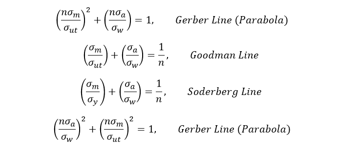
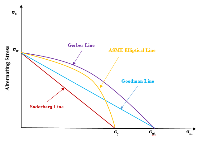
Figure 8: Mean Stress Correction Method
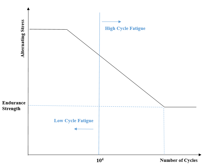
Low cycle Fatigue Vs High Cycle Fatigue:
The fatigue has been segregated into two region such as High cycle fatigue and Low cycle fatigue. The main difference between both is the number of cycles, elastic and plastic deformation behavior.
- Low Cycle Fatigue: The low cycle fatigue is characterized by repeated plastic deformations in each cycles. For example, if tensile load is applied to component until it plastically deformed, that would considered as one half cycle of LCF and in order to complete a full cycle part needs to deformed back to its original shape. Hence, the number of cycle that part can withstand before failure is much lower than the regular fatigue. In this, loading that typically causes failure in less than 104 cycles.
- High Cycle Fatigue: The high cycle fatigue is characterized by elastic deformation & the number of cycles to failure is high. HCF require more than 104 cycles to failure where stress is low and primarily elastic.
The transition life between LCF and HCF is determined by stress level (transition between plastic and elastic deformations). This transition life mainly depends on ductility of the material. E.g. 104 as shown in Figure 9.
Rainflow Cycle Counting:
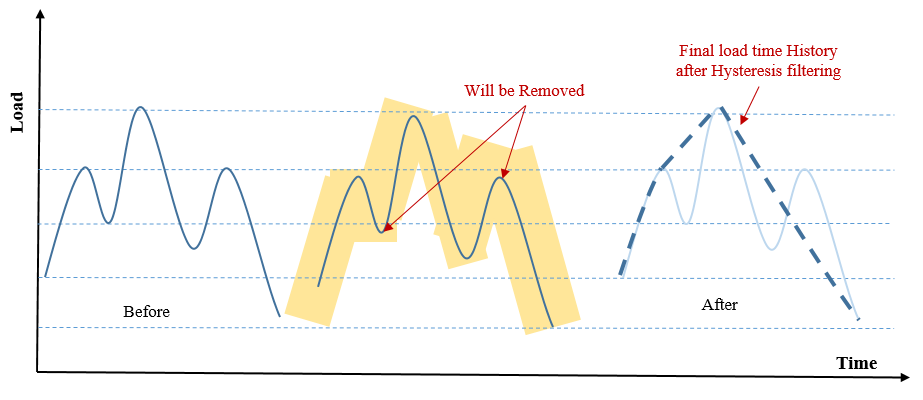
It is an algorithm that converts an irregular stress history or spectrum of varying stress into blocks of simpler stress cycles (equivalent set of simple stress reversals) that can be used for fatigue calculations. Real life loading is not necessarily cycle and often appears to be varying (random or transient) in nature, for which the number of cycles and their amplitudes does not easily determined. Rainflow counting is then used to extract the number of cycles, and their respective range and mean. Tatsuo Endo (Japan)and M. Matsuishi first introduce rainflow counting in 1967-68 and in 1986 the first rainflow counting standard, E1049 was published. There are various method of Rainflow counting; main four methods are mentioned below:
- Hysteresis Filtering
- Peak-Valley Filtering
- Discretization
- Four Point Counting Method
Fatigue Strength Reduction Factor (kf):
This factor is used to account the corrosion, surface finish, size factor, notch effect and various other surface irregularities. This is also referred in few international codes to calculate the fatigue life such as ASME; which states that, Fatigue strength Reduction factor is a stress intensification factor which accounts for the effect of a local structural discontinuity (stress concentration) on the fatigue strength. It is the ratio of the fatigue strength of a component without a discontinuity to the fatigue strength of that same component with a discontinuity.
Fatigue Analysis Outputs:
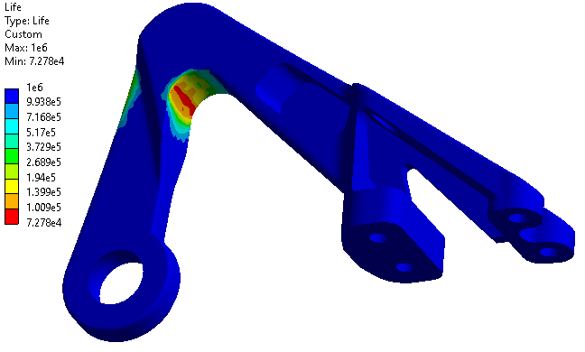
Fatigue Life:
Fatigue life is the available life for the given fatigue analysis. The analysis contour results shows the number of cycles until failure due to fatigue. Fatigue Life can be over the whole model or on parts, surfaces, edges, and vertices. If loading is of constant amplitude, this represents the number of cycles until the part will fail due to fatigue. If loading is non-constant, this represents the number of loading blocks until failure. Figure 11 shows the fatigue life of bracket, in this the maximum life shown is 1e6 is corresponds to maximum cycle to failure in SN curves and 7.27e4 corresponds to the region (red colour) of minimum life cycles.
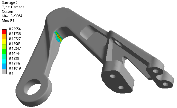
Fatigue Damage:
Fatigue damage is defined as the design life divided by the available life. For Fatigue Damage, values greater than 1 indicate failure before the design life is reached.
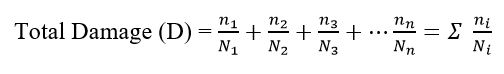
Damage Accumulation (Cumulative Damage):
In this Miner’s Rule is applicable; which assumes that the total damage is simply the linear summation of the partial damages:
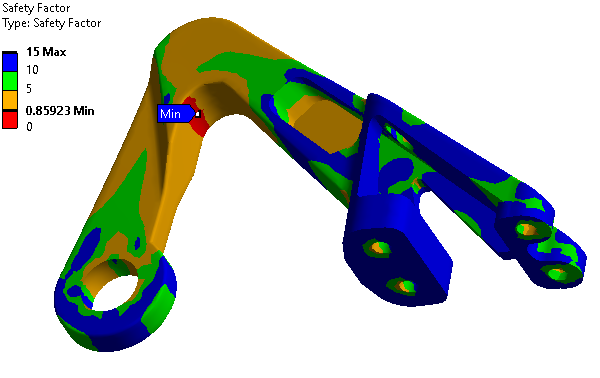
Safety Factor:
Fatigue Safety Factor is a contour plot of the factor of safety with respect to a fatigue failure at a given design life. For Fatigue Safety Factor, values less than one indicate failure before the design life is reached and the maximum factor of safety displayed is 15.
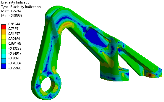
Biaxiality Indication:
Biaxiality indication gives the user some idea of the stress state over the model and how to interpret the results. Real world stress states are usually multiaxial. Biaxiality indication is defined as the principal stress smaller in magnitude divided by the larger principal stress with the principal stress nearest zero ignored. A biaxiality of zero corresponds to uniaxial stress a value of -1 corresponds to pure shear, and a value of 1 corresponds to a pure biaxial state.
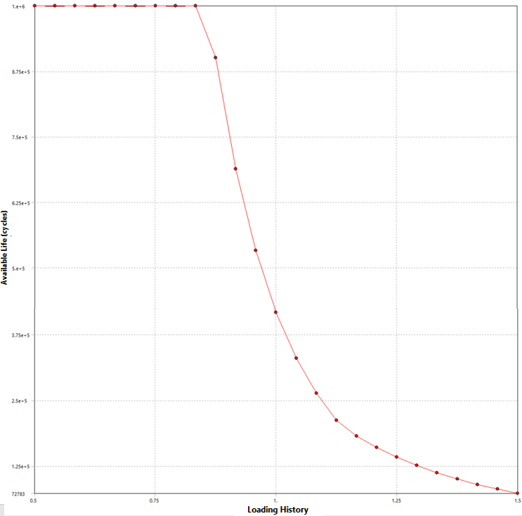
Fatigue Sensitivity:
It shows how the fatigue results such as life, damage, or safety factors varies as a function of the loading at the critical location on the model. The user may set the number of fill points as well as the load variation limits. For example, the user may wish to see the sensitivity of the model’s life if the FE load was 50% of the current load up to 150% of the current load.
References:
- https://en.wikipedia.org/wiki/Fatigue_(material)
- https://community.sw.siemens.com/
- ANSYS Manual